Figures
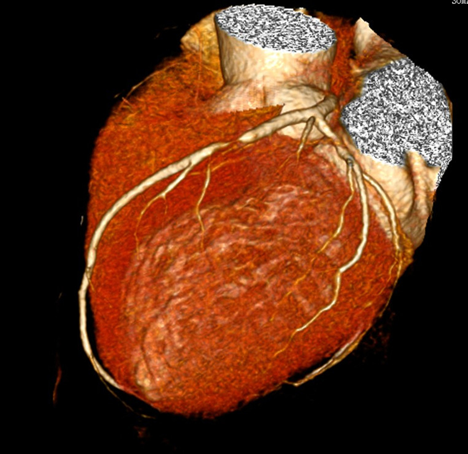
Figure 1. Patient of case 3 was male and 60 years old. CCTA showed severe stenosis of 90% in the proximal segments of LAD.
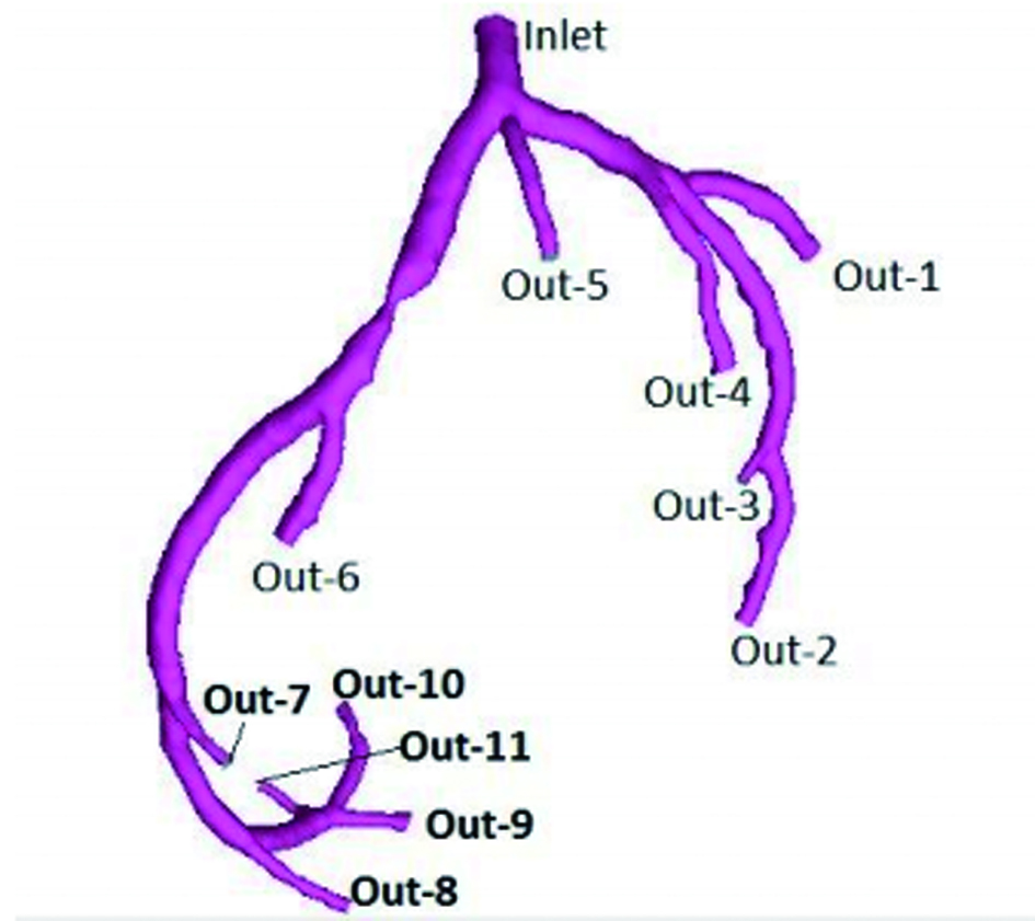
Figure 2. Patient of case 3 was male and 60 years old. Three-dimensional luminal model of the left coronary arteries was generated in software Mimics. Inlet was defined as entry of flow. Out-1 to Out-11 were set as free flow boundary.
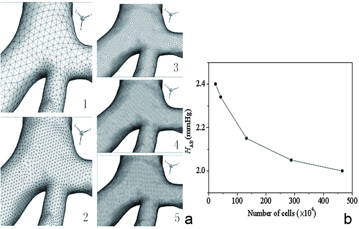
Figure 3. Part of the diagram of five kinds of densities of mesh of case 2 (a). The total number of grid ranged from about 240,000 to 4,660,000. The relationship between overall numbers of grid and computation which was described in a graph (b): overall numbers as abscissa and pressure descending of the LAD as ordinate. Pressure gradient change was in line with the trend of overall numbers of grid and differences were getting smaller.
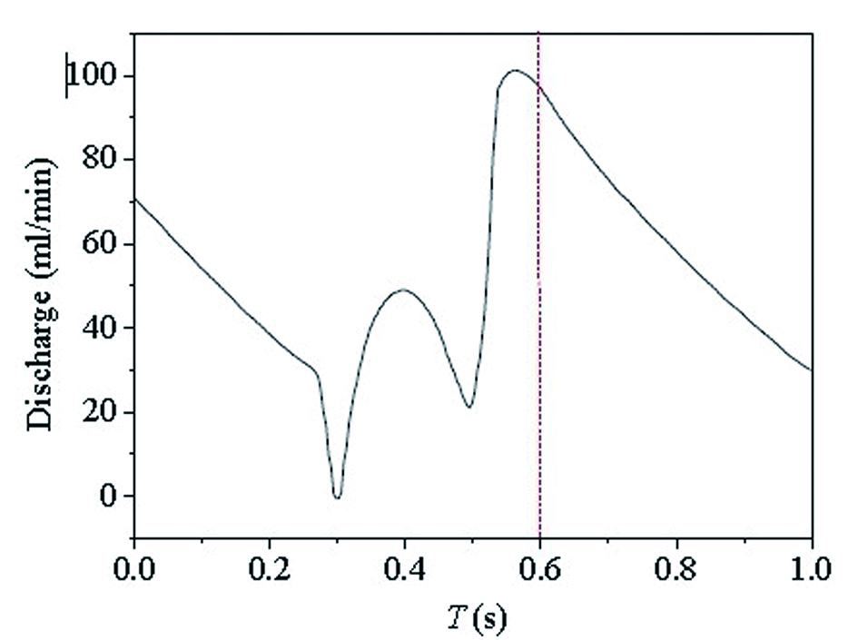
Figure 4. The graph of coronary arteries flow changes during cardiac cycle was reported by Chaichana et al [2]: time as abscissa (s) and quantity of flow as ordinate (mL/min). Flow of the entry of the left coronary artery (inlet) at different moment could be acquired.
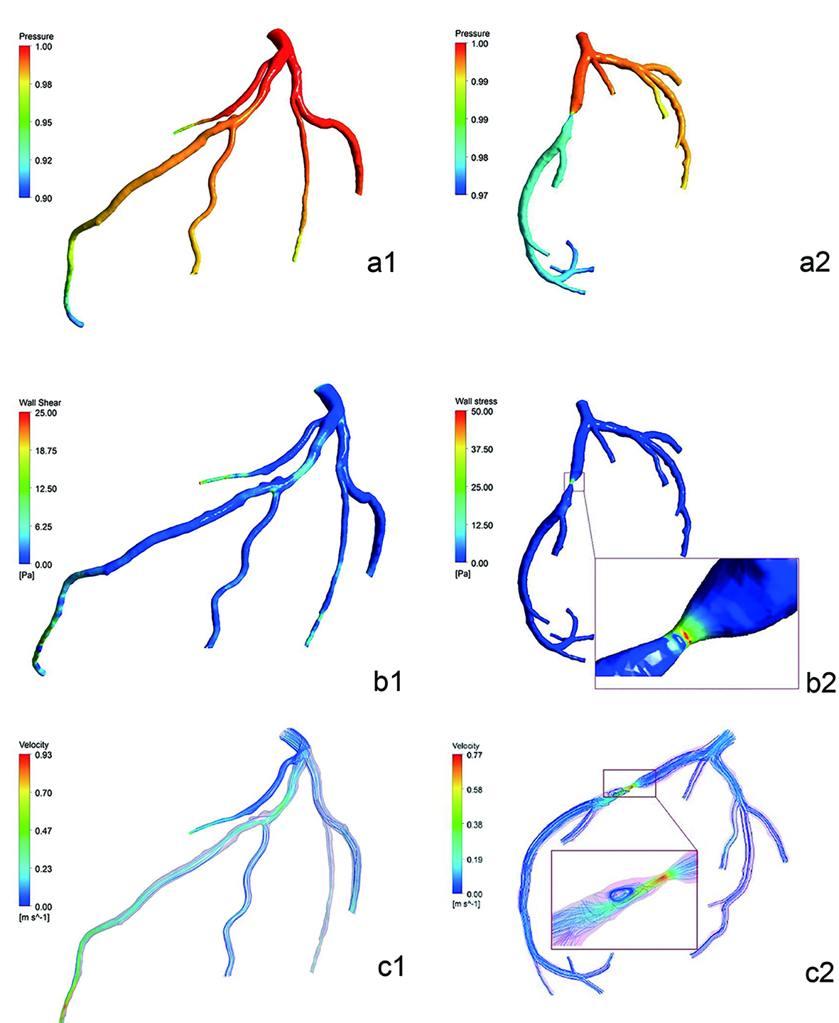
Figure 5. Pressure distribution simulated diagram of cases 2 and 3 (the entry was one) (a1-a2). There was little descending in the pressure gradient of case 2. But the descending in the color difference which was pressure gradient of case 3 between proximal and distal of stenosis of LAD was large. Noteworthy reduction of pressure was observed in the distal segment of left septal branch of case 2. It showed the WSS distribution simulated diagram of cases 2 and 3 (Pa) (b1-b2). WSS values in lumen without plaques or stenosis were low and uniform. At regions opposite to the flow divider, dominant low WSS values occurred. In case 3, WSS values of severe stenosis were higher. It showed the flow velocity distribution simulated diagram of cases 2 and 3 (m/s) (c1-c2). Blood flow velocity distributed uniformly in the LAD, and center axial flow was faster than border flow. Blood flow velocity gradient barely changed in the stenosis segment of case 2. But there was obvious variation in LAD of case 3: acceleration of flow velocity on both ends of stenosis, the fastest flow velocity in the center of stenosis, obvious turbulence after end of stenosis.
Table
Table 1. Comparison of the Mean Values of Flow Pressure Gradient and CER in the LAD of Three Cases (x ± s)
| LAD | Case 1 | Case 2 | Case 3 |
|---|
| Flow pressure gradient | CER | Flow pressure gradient | CER | Flow pressure gradient | CER |
|---|
| Proximal segment | 1.00 ± 0.0000 | 0.98 ± 0.0082 | 1.00 ± 0.0000 | 0.99 ± 0.0245 | 1.00 ± 0.0000 | 0.99 ± 0.0082 |
| Middle segment | 0.98 ± 0.0082 | 0.96 ± 0.0141 | 0.98 ± 0.0163 | 0.96 ± 0.0082 | 0.98 ± 0.0082 | 0.89 ± 0.0141 |
| Distal segment | 0.96 ± 0.0216 | 0.93 ± 0.0216 | 0.94 ± 0.0163 | 0.95 ± 0.0216 | 0.90 ± 0.0141 | 0.93 ± 0.0141 |
| Proximal end of stenosis | - | - | 0.99 ± 0.0082 | 0.99 ± 0.0245 | 0.98 ± 0.0163 | 0.93 ± 0.0216 |
| Distal end of stenosis | - | - | 0.98 ± 0.0082 | 0.97 ± 0.0141 | 0.92 ± 0.0163 | 0.80 ± 0.0283 |